Fractal PCA Image Compression: An Exploration

Over the summer, I tinkered with DCT-based image compression after watching a Computerphile video. For me, the intersection of linear algebra, programming and art made it deeply fascinating and gave me a deeper interest into signal processing in general. This article is a little story of what I made along the way while playing around with some code and math I found enthralling.

The exploration gave me a new understanding of matrices, as I understood how they were actually applied in a real problem. Breaking apart the elegance of using dot products to derive coefficients led to an interesting and satisfying proof. The proof ultimately boils down to the fact the basis vectors are orthonormal. Before embarking on this journey, you would’ve lost me at “orthonormal” and “eigenvector”, it’s been a super interesting one.

FYI: If you have no prior knowledge of the DCT and how JPEG image compression works, this article will probably be unenjoyable. I suggest watching the Computerphile video, and educating yourself on some of the terms used. I would love to write an introduction and explanation of the DCT myself, but its quite a lot of work and I’m an IB student.

The Journey to Understanding the DCT

Initially, I was curious as to how the coefficients for each 8x8 image patch were computed. I could wrap my head around the idea that any image block could be reconstructed by summing sine waves from my prior understanding of the Fourier Transform. But 3 things stuck out to me:

• Doesn’t a perfect reconstruction require an infinite amount of waves, to perfectly recreate a signal?
• Tangential to my first question was: How can we be sure that just these 8 basis vectors could create any possible image / signal?
• How do we find the right set of coefficients to recreate an image patch or signal?

These three questions threw me deeper into the rabbit hole.

To solve the first 2, an answer to either one would actually be suitable answers for both. So, I could delve into some complex math, but thats a little too clinical, and its not how I learn. So I’ll tell you the logical and intuitive journey that I took to understanding these questions.

I first dug and found out that actually, with the right basis vectors, or initial set of waves, any pattern could be recreated. Okay, but how and why? Google told me it was because of “orthonormality”. I learnt it meant that each set of basis vectors were both “orthogonal”, meaning at right angles with each other and “normal” meaning having a length of one. The intriguing part for me was trying to wrap my head around how a 64 different vectors could be all 90 degrees apart from each other. The most I could imagine was the normals pointing out of a cube, but that’s only 6, and actually, some of the vectors are 180 degrees apart. But this way of thinking about it opened a solution for me.

I found it helpful to imagine a simplified set of basis vectors, just 2 dimensions. In 2D, it is possible to point to any place with a set of 2 numbers, the x and y coordinates, essentially “how far right” and “how far up”. The important part to though, was that this is only possible because the directions had some angle between them. For the DCT basis vectors, having 90 degrees between them means they can most optimally represent and cover the space. I began thinking of each possible 8x8 image patch as a point in a 64 dimensional space. And because of the orthogonality, just like in 2D, every point can be described with a set of 64 coordinates. I found it interesting how extending the geometry of the 3D world that we’re used to, is unexpectedly intuitive; all the same rules and notions of orthogonality, direction, dot products, etc. carry over into higher dimensions rather intuitively.

So that answered the first 2 questions quite soundly for me: Doesn’t a perfect reconstruction require an infinite amount of waves, to perfectly recreate a signal? and How can we be sure that just these 8 basis vectors could create any possible image / signal? We only need 64 coordinates, because each of the 64 basis vectors is completely orthogonal, and can represent any point possible in our 64 dimensional space, ensuring coverage.

And by the way, there are an infinite amount of orthonormal basis vectors that we can come up with. The most basic probably being: [1, 0, 0, 0, ..., 0], [0, 1, 0, 0, ..., 0], [0, 0, 1, 0, ..., 0]. With these basis vectors reconstructing any signal seems trivial. Yes, the coefficient for each basis vector is just it’s coordinate. But, see that’s not a transform. That really clicked for me. I realized its called a transform because you are writing it in a different set of coordinates. And for JPEG compression, you break it apart into frequency, which becomes very useful when you want to remove data that doesn’t make very visible change. If we didn’t write each patch as combination of progressively higher frequency patterns, how could we find what part of the image’s data to remove?

While pondering about how I may solve this last question, I wanted to apply a technique I already knew: gradient descent. I sort of framed finding the right coefficients as an optimization problem, where the objective is to minimize the difference between he reconstructed image and original. But, while going through the math to derive the gradient function (derivative) of the cost function, it led down a path that revealed a, all that was required was just a dot product. Furthermore, I realized solving for the minimum was extremely trivial, and was effectively the inverse of the matrix of basis vectors, B times the signal, v: C = B^Tv, to yield C the list of coefficients.

Furthermore, the inverse of an orthonormal matrix is actually its transpose (that ones a fun one to prove, you should give it a try). Going through the math, you realize finding the coefficients is actually just doing a dot product for each basis vector and the signal. This made sense, as any signal that is completely perpendicular to a basis vector should have none of its component in it. The behavior we want is exactly what a dot product gives.The elegance and surprise of seeing both seemingly very different and abstract methods converge reminded me of the beauty of mathematics.

Experimenting with Custom Basis Vectors

At this point, I was so enthralled with the DCT, I kept learning everything I could about it. Soon, I had my own ideas. One of them being to not use the same DCT basis vectors for every image, but instead create 64 basis vectors that were optimized at capturing the most energy (energy density) as possible. In layman’s terms, its capturing the most perceptually important detail in the fewest amount of coefficients. With gradient descent still lingering in my mind, I tried to use it to construct these per-image basis vectors.

The methodology was to:

• Representing the 64 basis vectors as a 64×64 list
• Each iteration, incrementally bump each pixel by slightly up or down, depending on which direction increased the energy compaction metric
• One large issue was that the dot product trick of finding coefficients didn’t work as well, because the vectors from this method weren’t guaranteed orthonormality.
• However, to my delight the algorithm pulled through somewhat and created cool, natural-looking shapes and basis vectors. Though I had hoped for a smaller file size, these performed much worse than DCT.

The night that I was programming my gradient descent experiment, was the night before a 5 a.m in the morning. I left my gradient descent to optimize, running all night and wound up not sleeping at all that night. However, as soon as I boarded the plane, I didn’t open an eye until after five hours.

Discovery of PCA

After waking up, I began talking to my seat neighbor. Our conversation began going towards talking about university and then to math. Turns out the guy was a pretty big math nerd. I excitedly brought up the DCT and why I thought it was interesting. I hadn’t realized how closely linked his work was to mine at the time, when he showed some image processing experiment he had been fiddling with. He brought out his phone and shows me an image of the Mona Lisa reconstructed using a single eigenvector. You could see the basic colors and resemblance immediately, however, as he added more and more eigenvectors in the reconstruction, finer and finer detail on her face began to appear. I didn’t know it, but the math behind his artistic experiment happened to be the very solution to solving my problem of finding per-image-optimized basis vectors. Of course, I showed him own tinkerings, the prototype I worked on all night. He was interested, and suggested I take a look at PCA, the same math behind how his demo worked as that might be solution.

Even writing about this encounter makes me feel like its a fairytale. I can’t believe the odds of finding a solution to a problem I had been working on all night, next to a guy I just met on my flight.

After the flight, I did some reading on PCA and eigenvectors, but the idea didn’t click for me, until I had this revelation: if we could somehow look at all the 8×8 patches in an image, and somehow have some method of extracting the most common pattern, some highest common denominator or component of every 8x8 patch. This is how PCA clicked for me. Essentially, if we plot every single 64 dimensional data point (each patch has one), we would see clusters of points, their general area is the vector we want to extract. That’s a grossly simplified metaphor, but the image just stuck in my head. PCA finds the “direction” in this 64D space that maximizes the sum of dot products, essentially looking for the most “aligned” direction. That’s our first common denominator, the basis vector with the highest average coefficient. To find all 63 other basis vectors, we remove that first direction and find the next one. Continuing this leads us to find all our basis vectors. This is PCA in action and its how the Karhunen–Loève transform works. Fun fact actually, the KLT came out before the DCT, but it was too expensive to compute, and impractical. So, ironically, while looking for a better compression method, I arrived on the precursor to the DCT.

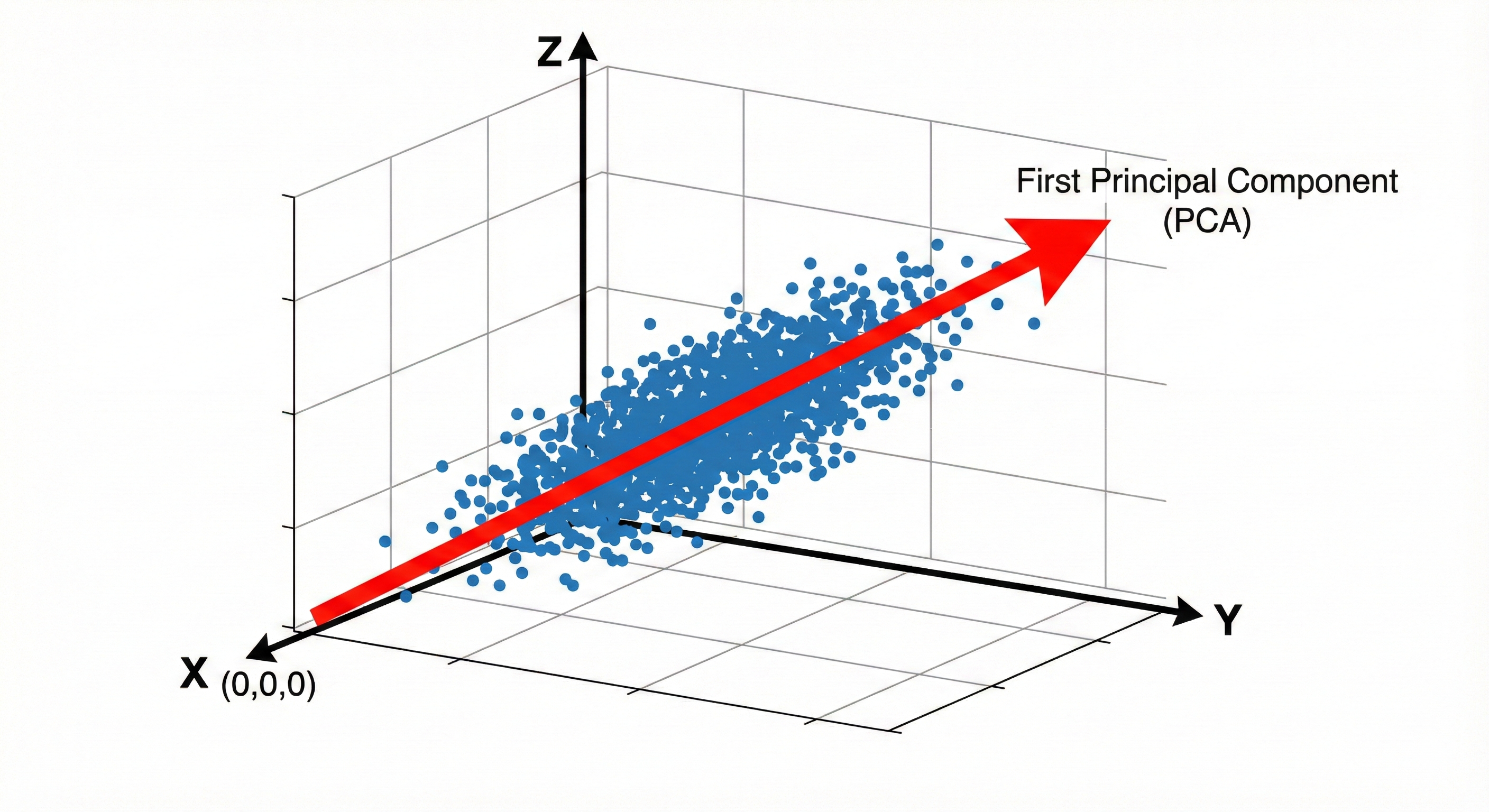
Above: Each point is a 8x8 patch, the red arrow represents the most common / shared signal, that’s the first principal component (Generated with nano banana pro)

Also, another one of those brilliant nuggets of elegance: The basis vectors derived from this PCA method, actually are orthonormal. (I’ll leave why this is, as an exercise to the reader)

Let me show this in action, we’ll use this image to demonstrate:

Now, after doing PCA on the image above to derive each basis vector and representing them as an 8x8 images in a zig-zag pattern from the top left to bottom right, results in this:

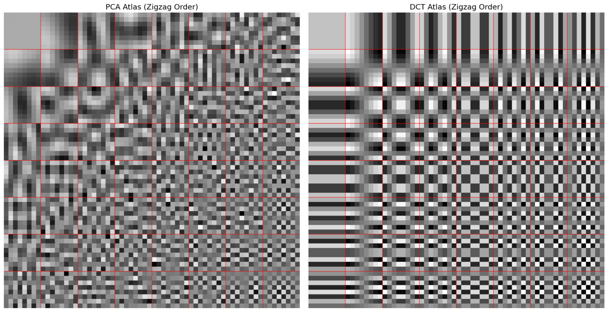
On the left is the PCA derived basis vectors, and the right has the standard DCT basis vectors. You can notice how higher-frequency basis vectors are in the bottom-right corner, just like with the DCT, and how the first few vectors capture low-frequency natural shapes. I kept the top-left DC value locked at grey to recenter the entire dataset from the start.

I was excited to see how much more energy compact and data efficient this new method was. But seeing how similar DCT and PCA basis vectors already were didn’t give me much confidence. It turns out, DCT’s basis vectors do an amazing job at compacting energy in natural images. However, I was still curious if the additional data required to store the PCA basis vectors themselves would be greater that the space savings from the slightly more optimal energy compaction.

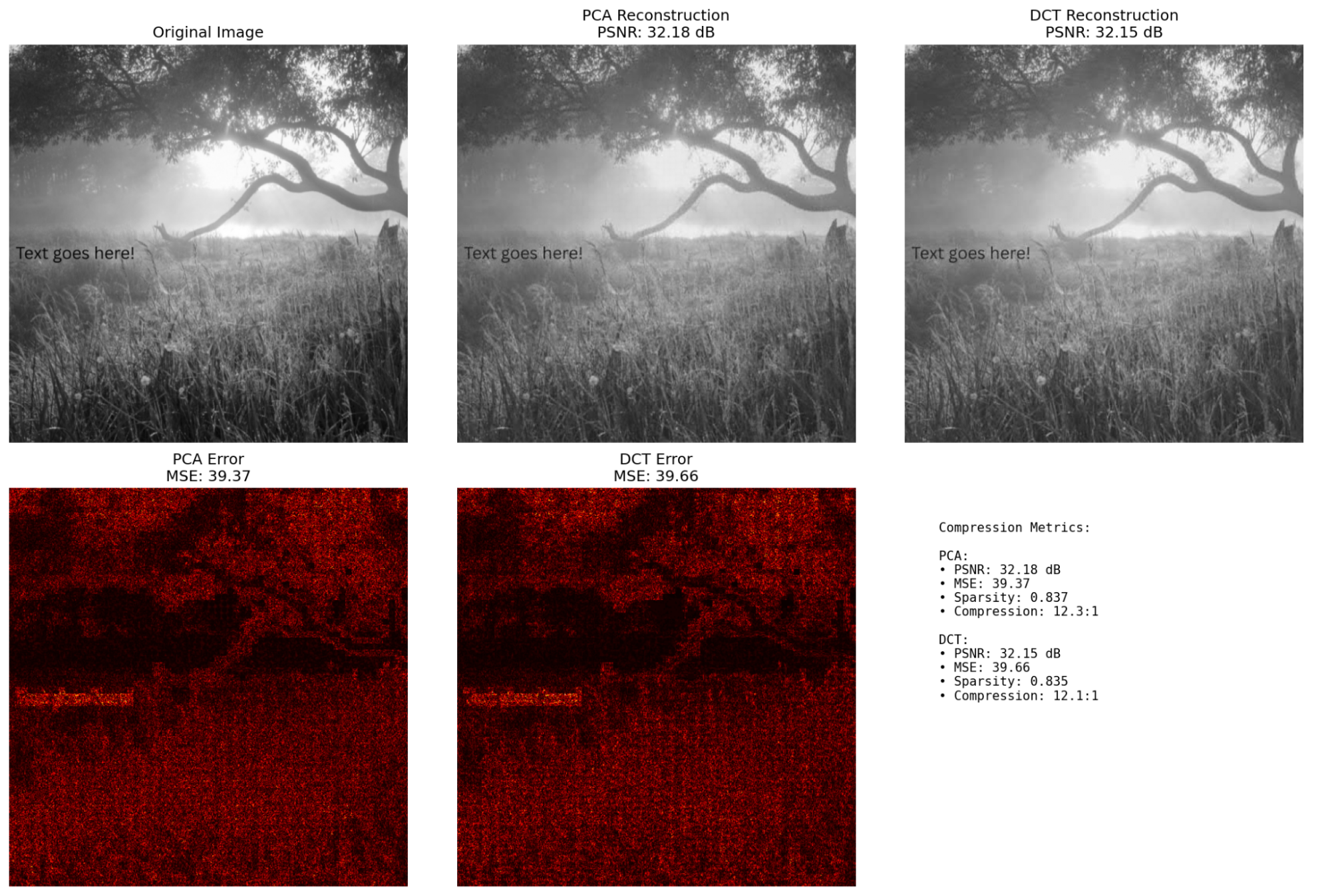
However, after some testing, I found out that the DCT performs the same visually for the same file size. I guess that explains why DCT hasn’t been reinvented for 30 years.

Yet I wasn’t discouraged by this result. After some more rumination and experimentation, the idea of using a variation of different sized patches (apart from just 8x8) seemed like a promising endeavor. After evolving this idea, I thought, what if we adaptively use smaller patches for regions which need more detail and use larger patches for regions of low-frequency detail, while incorporating PCA (over DCT to keep image fidelity)?

A Hierarchical Approach

So I came up with this clean and refined explanation of my proposed compression algorithm:

“A multi-scale hierarchical PCA compression framework that learns optimal orthogonal bases at varying block sizes—2×2, 8×8, 32×32, etc.—and adaptively prunes the hierarchy by merging finer blocks into coarser ones using nearest PCA atlas approximations. This approach balances energy compaction and bitrate overhead, enabling efficient, data-driven image representation that flexibly captures local detail while minimizing storage costs.”

After doing some research, I figured that this could be very useful specifically for medical imagery. The adaptive resolution style compression would allow empty (black) portions of an X-ray or other medical image to use less information, while detailed sections could use the highest resolution detail.

Reality Check

However, after lots of testing, I ran into some limitations of my method. PCA wasn’t justifiably superior to DCT and the fractal arrangement caused abrupt changes in resolution between fragments of the image that use different sized blocks. Additionally, serializing this tree structure and the resolutions of each fractals was quite a complex undertaking, and without proper optimization, it took too much data. And of course, storing the basis vectors for a 16x16 atlas and smaller wasn’t practical.

Either way, I thought the results were fascinating, so here’s a few screenshots from the testing.

Above: The reconstructed image using this compression technique

Above: Here’s the basis vectors, but for each resolution of patch size

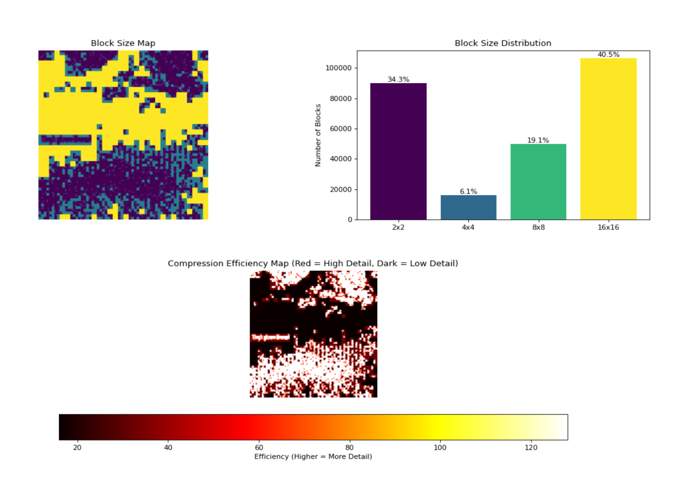
Above: In the top left there’s the block size map, showing parts of the image and the block size they used. Top right shows the distribution of block sizes. What’s pretty cool is that discouraging smaller blocks is neat because it’s essentially a compression aggressiveness slider. Notice how the higher detail grass and leaves are filled with small blocks, while the sky and gradient sections use larger blocks

Conclusion

All in all, going through learning the math, coming up with ideas, implementing them in code and developing them, then testing viability and repeating this process was extremely fun and fulfilling and gave me a massive amount of understanding for matrices, compression, signal processing, optimization, transforms and linear algebra in general. Although in the end my work didn’t culminate into anything that was groundbreaking, I ended up using this to create my own image file format, called “.xvp”. And although it is about ten times the size of an equivalent PNG, and about 50× the size of an equivalent quality JPEG, I’m still proud of it.

There’s just one thing I wished I tried though. I realized perhaps storing a set of basis vectors for each patch size (2x2, 4x4, 8x8, 16x16) might not be necessary. Perhaps its possible to reconstruct the 8x8, 4x4 and 2x2 maps just with the 16x16. Let me know if you have a solution.